Introduction

The MNIST data set is the “Hello World” of deep learning and computer vision. It consists of images of handwritten digits (from 0 to 9) and their associated labels (the actual digits represented). The challenge is to develop an algorithm that looks at an image and tells us what digit is in it. This is a classification problem with 10 classes.

The standard approach in supervised machine learning is to first let the algorithm learn the relationship between images and labels using a training data set and then assess how well it performs with images that it has never seen before.

GalaxyMNIST

While the MNIST data set is a very good first place to get started hands on with machine learning, I find it beautiful to have alternative options such as the GalaxyMNIST dataset.

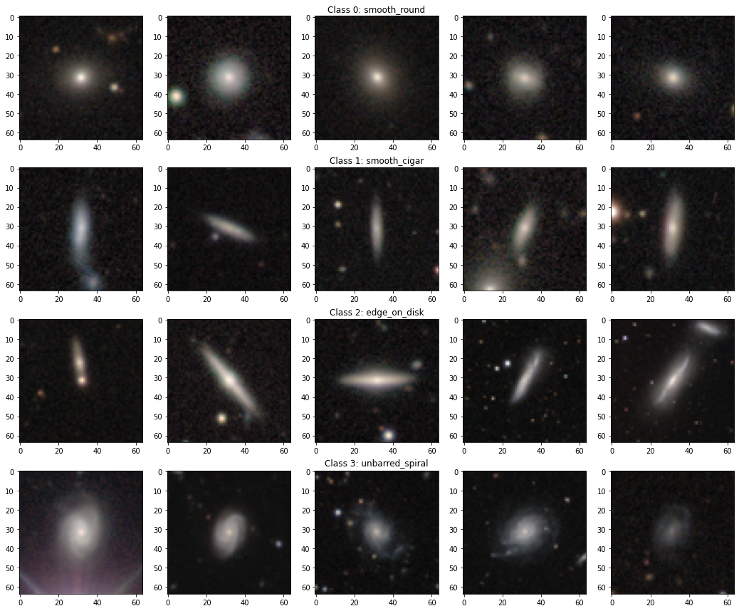
The GalaxyMNIST is a data set of 10.000 images of galaxies labeled as belonging to one of four morphology classes (assigned manually by Galaxy Zoo volunteers, check out this and other super cool projects in Zooniverse!). Each image contains 3x64x64 pixels (RGB color, width, height).

The four glaxy classes are:

smooth_round
smooth_cigar
edge_on_disk
unbarred_spiral.

Below are some examples for each class in the different rows:

The intention of this post is mostly to let others know of the existence of GalaxyMNIST rather than explaining my very simple solution to the problem.

The challenge

The challenge is to train a machine learning model (using the train data set) that learns the relationship between the images and the 4 possible labels. The test data set is used to compare predicted labels with actual ones and to measure the model accuracy.

This notebook is the result of a 2-hour hack session in the Institute of Cosmology and Gravitation (thanks Coleman for the session and putting up the notebook to get started!). All the results were obtained in this time frame (afterwards I just did some polishing).

The Solution

See the full solution in this Colab notebook (in Python + Keras):

https://colab.research.google.com/drive/1LmNlgNPl3PNBWuOsBZCB4-DfhB7YX6v1?usp=sharing

Given the time constraints, I chose a very simple strategy. I adapted a solution to the original MNIST problem found in this notebook of Google’s Machine Learning Crash Course.

I used a simple neural network of fully-connected layers with 3 hidden layers. A Convolution Neural Network would be much more suited, because it would preserve spation information. Again, the goal was to get something working in less than 2 hours!

Loading in the data set

GalaxyMNIST inherits from the original MNIST, and the training and test data can be loaded in Colab as follows:

%pip install git+https://github.com/mwalmsley/galaxy_mnist.git
from galaxy_mnist import GalaxyMNIST

dataset = GalaxyMNIST(
    root='/galaxy_mnist_download',
    download=True,
    train=True
)

testset = GalaxyMNIST(
    root='/galaxy_mnist_download',
    download=True,
    train=False
)

display(dataset)
display(testset)

Dataset GalaxyMNIST
Number of datapoints: 8000
Root location: /galaxy_mnist_download
Split: Train

Dataset GalaxyMNIST
Number of datapoints: 2000
Root location: /galaxy_mnist_download
Split: Test

Images are in dataset.data with shape [8000, 3, 64, 64].

Labels are in dataset.targets with shape [8000].

Labels are numbers 0-3, corresponding to dataset.classes: [‘smooth_round’, ‘smooth_cigar’, ‘edge_on_disk’, ‘unbarred_spiral’]

Normalize the images

The images come as grayscale values between 0-255 for each rgb channel that we want to normalize to the range 0-1:

x_train = np.array(dataset.data[:,:]/255.0)
x_test  = np.array(testset.data[:,:]/255.0)
y_train = np.array(dataset.targets)
y_test  = np.array(testset.targets)

Neural network architecture

We start by first flattening the array, which is then passed to the neural network. There are three hidden layers with 512 neurons and the output layer corresponds to the 4 classes:

[3,64,64] - [12288] - [512] - [512] - [512] - [4]

We make use of dropout, relu and softmax functions.

def create_model(my_learning_rate):
  """Create and compile a deep neural net."""
  model = tf.keras.models.Sequential()

  # Flatten the 3x64x64 array into a a one-dimensional array.
  model.add(tf.keras.layers.Flatten(input_shape=(3, 64, 64)))

  # Hidden layers and dropout regularization layers
  model.add(tf.keras.layers.Dense(units=512, activation='relu'))
  model.add(tf.keras.layers.Dropout(rate=0.2))

  model.add(tf.keras.layers.Dense(units=512, activation='relu'))
  model.add(tf.keras.layers.Dropout(rate=0.2))

  model.add(tf.keras.layers.Dense(units=512, activation='relu'))
  model.add(tf.keras.layers.Dropout(rate=0.2))

  # Output layer, 4 classes
  model.add(tf.keras.layers.Dense(units=4, activation='softmax'))     

  # Create model
  model.compile(optimizer=tf.keras.optimizers.Adam(lr=my_learning_rate),
                loss="sparse_categorical_crossentropy",
                metrics=['accuracy'])

  return model    

Train the model

Finally, we just need to set some hyperparameters and train the model:

def train_model(model, train_features, train_label, epochs,
                batch_size=None, validation_split=0.1):
  """Train the model by feeding it data"""

  history = model.fit(x=train_features, y=train_label, batch_size=batch_size,
                      epochs=epochs, shuffle=True,
                      validation_split=validation_split)

  # Gather a snapshot of the model's metrics at each epoch.
  epochs = history.epoch
  hist = pd.DataFrame(history.history)

  return epochs, hist    

# Hyperparameters
learning_rate = 0.0015
epochs = 50
batch_size = 1000
validation_split = 0.2

my_model = create_model(learning_rate)

epochs, hist = train_model(my_model, np.array(x_train), np.array(y_train),
                           epochs, batch_size, validation_split)

Results

Accuracy

The accuracy of this simple neural network gets better as the training phase progresses and it seems to flatten after about 50 epochs:

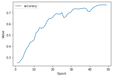
The accuracy on the test set is 70%. Note that the four classes contain a similar number of examples (if there was an imbalance, the accuracy would not be very informative).

Confusion matrix

The confusion matrix shows the relationship between actual and predicted classes:

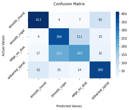
An exact solution would result in a diagonal confusion matrix, with zero cases off the diagonal. Note that the classes smooth_round and unbarred_spiral are often classified correctly, while the performance is worse for smooth_cigar and edge_on_disk, and often these two classes are confused. This is not surprising at all if we look again at the example galaxies displayed earlier, as these two classes contain elongated galaxies and look very similar.

Final notes

It was fun to learn about the GalaxyMNIST data set in this hack session. I hope you found it interesting too! Can you implement a solution that reaches a better accuracy?

Galaxy MNIST